In the bottom of that sidebar, you find pictures and videos of my beautiful Colombia! Enjoy it!

Sudoku!

This is one of my hobbies. I share with you becouse is a good way to distract you of stress from University or School! I hope you like it! Oh, I'll give to you a little advice: When you finish it, please go back to study numerical methods.
El sudoku del día por SudokusWeb.com

Monday, July 26, 2010

Excell's Templates

.
Hi, if you want a see or use some of my templates, here they are!
Just, download for a view in Excell's format

TEMPLATE 1
Contents: Bisection method, linear interpolation, Newton Raphson's method, Secant method and substitution


Autor: Carlos Andrés Uribe Hidalgo


TEMPLATE 2
Contents: Fixed point


Autor: Marcela Andrea Carrillo
 

TEMPLATE 3
Contents: Fixed point, Secant method, bisection method, false position method and Newton Raphson's method


Autor: Luis Carlos Molina, Brian Leonardo Gil


TEMPLATE 4
Contents: Secant method and Newton Raphson's Method


Autor: Arcadio Cuy

Sunday, July 25, 2010

Cholesky decomposition

:

Sunday, July 18, 2010

LU Descomposition and matrix inversion

-
LU Descomposition

Although is certianly represents a sound way to solve such systems, it become inefficient when solving equations with the same coefficients [A], but with different rignt-hand-side constants (the b's). Recall that Gauss elimination involves two steps: foward elimination and backsubstitution. Of these, the foward elimination step comprimeses the bulk of the computational effort. This is a particulary true for large systems of equations. LU descompositions methods separate the time - consuming elimination of the matrix [A] from the manipulations of the right side hand vectors can be evaluated in an efficient manner. Interestingly, Gauss elimination ifself can be expressed as LU descomposition. Before showing how this can be done, let us a first provide a mathematical overview of the descomposition strategy.

Overview of LU Descomposition

Just as was the case with Gauss elimination, LU descomposition requires pivoting to avoid division by zero. However, to simplify the following description, we will defer the issue of pivoting until after the fundamental approach is elaborated. In addition, the following explanation is limited to a set of three simultaneous equations. The results can be directly extended to n-dimensional systems.

[A] {x} - {B} = 0 (1)

Suppose that equation (1) could be expressed as an upper and triangular system

(2)

Recognize that this is similar to the manipulation that occurs in the first step of Gauss elimination. That is, elimination is used to reduce the system to upper to triangular form.Equation (2) can also be expressed in matrix notation and rearrange to give,

[U][X]-[D]=0 (3)

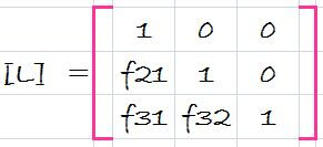
Now, assume that there is a lower diagonal matrix with 1's on the diagonal,

(4)

that is the property that when the equation (3) is premultiplied by it, equation (1) is the result.

That is,
[L]{{U}{X} - {D}}=[A]{X} - {B} (5)

If this equation hold, it follows from the rules of matrix multiplication that

[L][U]=[A] (6) and [L][D]=[B] (7)

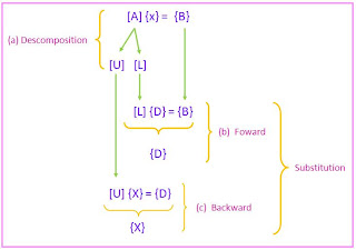
A two step strategy for obtaining solutions can be based on equations (3) (6),and (7)
  1. LU descomposition step. [A] is factored of "descomposed" into Lower [L] and Upper [U] triangular matrices.
  2. Substitution step- [L] and [U] are used to determine a solution {X} for a right hand side {B}. This step ifself consists of two steps. First, equation (7) is used to generate an intermediate vector {D} by forward substitution. Then, the result is substituted into the equation (3), wich can be solved with back sustitution for {X}.


LU Decomposition Version of Gauss Elimination

Although it might appear at face value to be unrelated to LU decomposition, Gauss elimination can be used to decompose [A] into [L] and [U]. This can be easily seen for [U], which is direct product of the forward elimination. Recall that the forward-elimination step is intended to reduce the original coefficient matrix [A] to the form

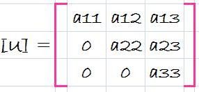
wich is in desired upper triangular format.

Though is might not be as apparent, the matrix [L] is also produced during the step. This can be readily illustrated for a three-equations system,


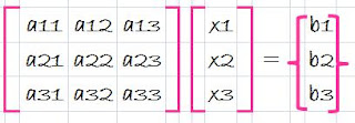
The first step in Gauss elimination is to multiply row 1 by the factor [recall Eq. 12]

f21= a21/a11

and substract the result from the secoond row to eliminate a21. Similarly, row 1 is multiplied by

f31=a31/a11

and the result subtracted from the third row to eliminate a31. The final step is to multiply the modified second row by

f32= a32/a22

and subtract the result from the third row to eliminate a32.

Now suppose that we merely perform all these manipulations on the matrix [A]. Clearly, if we do not want to change the equation, we also have to do the same to the right-hand side {B}. But there is absolutely no reason that we have to perform the manipulations simultaneously. Thus, we could save the f's and manipulate {B} later.

Where do we store the factors f21, f31 and f32? Recall that the whole idea behind the elimination was to created zeros in a21, a31, and a32. Thus, we can store f21 in a21, f31 in a31, and f32 in a32. After elimination, the [A] matrix can therefore be written as


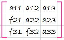
This matrix, in fact, represents an efficient storage of the LU decomposition of [A],

[A] -> [L][U]
where
and

source: chapra 5th edition

Direct Methods For The Solution Of Systems Of Equations

-
The Engineer of Universidad Industrial de Santander, UIS, Bucaramanga, Colombia, Elkin Santafe, based in his knowledge and his research, give to us a little summary about direct methods for the solution of systems of equations

Newton Raphson Method

.
The most efficient method for finding a root of an equation is known as Newton-Raphson. In this method, instead of doing linear interpolation between two points known to straddle the root, as in the secant method, we use the value of the function g and its derivative g' at some point z, and simply follow the tangent to the point where it crosses the axis.


Obviously, zn = z - g(z)/g'(z). In this example, you can see that the next iteration (starting at zn) will already bring us very close to the root. When it can be used, Newton-Raphson converges extremely rapidly. In fact, the number of digits of accuracy doubles at each iteration. However, the method requires that we know g', which may not always be the case (for example, if g is known only as a tabulated or numerically defined function). Note, though, that it is possible to make numerical estimates of g' by evaluating g at two nearby points. The method also suffers from the fact that it can be wildly unstable if we start far from the root (for example, if we started at the point labeled z2 in the earlier figures, Newton Raphson would send us off in entirely the wrong direction). And of course, if happen to land near a turning point, where g'(z) = 0, the method will fail badly. Like the secant method, Newton-Raphson is often used to refine our results after bisection has already brought us fairly close to the desired solution.


Newton Video

:

Fixed point iteration

.

In numerical analysis, fixed point iteration is a method of computing fixed points of iterated functions.
More specifically, given a function f defined on the real numbers with real values and given a point x0 in the domain of f, the fixed point iteration is X n+1= f (Xn), n = 0,1,2,... which gives rise to the sequence Xo, X1, X2,... which is hoped to converge to a point x. If f is continuous, then one can prove that the obtained x is a fixed point of f, i.e.,

f(x) = x
More generally, the function f can be defined on any metric space with values in that same space.


*Method of False Position

.
The poor convergence of the bisection method as well as its poor adaptability to higher dimensions (i.e., systems of two or more non-linear equations) motivate the use of better techniques. One such method is the Method of False Position. Here, we start with an initial interval [x1,x2], and we assume that the function changes sign only once in this interval. Now we find an x3 in this interval, which is given by the intersection of the x axis and the straight line passing through (x1,f(x1)) and (x2,f(x2)). It is easy to verify that x3 is given by


Now, we choose the new interval from the two choices [x1,x3] or [x3,x2] depending on in which interval the function changes sign. The false position method differs from the bisection method only in the choice it makes for subdividing the interval at each iteration. It converges faster to the root because it is an algorithm which uses appropriate weighting of the intial end points x1 and x2 using the information about the function, or the data of the problem. In other words, finding x3 is a static procedure in the case of the bisection method since for a given x1 and x2, it gives identical x3, no matter what the function we wish to solve. On the other hand, the false position method uses the information about the function to arrive at x3.


Source: http://web.mit.edu/10.001/Web/Course_Notes/NLAE/mode5.html

*Bisection Method

.

My Colombia!