Excell's Templates

.

Hi, if you want a see or use some of my templates, here they are!

Just, download for a view in Excell's format

TEMPLATE 1

Contents: Bisection method, linear interpolation, Newton Raphson's method, Secant method and substitution

http://s3.amazonaws.com/ppt-download/plantillametodos-100727004936-phpapp01.xls?Signature=oc8Tdu4JMsAQ%2BsAjrwApR2TgUuM%3D&Expires=1280210248&AWSAccessKeyId=AKIAJLJT267DEGKZDHEQ

Autor: Carlos Andrés Uribe Hidalgo

TEMPLATE 2

Contents: Fixed point

http://s3.amazonaws.com/ppt-download/puntofijo-100727013552-phpapp01.xlsx?Signature=l9EcYr6VgQ%2FYv9KTNVjztBEuRx0%3D&Expires=1280213242&AWSAccessKeyId=AKIAJLJT267DEGKZDHEQ

Autor: Marcela Andrea Carrillo

 

TEMPLATE 3

Contents: Fixed point, Secant method, bisection method, false position method and Newton Raphson's method

http://s3.amazonaws.com/ppt-download/metododebiseccion-100727011748-phpapp01.xlsx?Signature=MU4sNyejwIqz7woSpanHIn9mR54%3D&Expires=1280211912&AWSAccessKeyId=AKIAJLJT267DEGKZDHEQ

Autor: Luis Carlos Molina, Brian Leonardo Gil

TEMPLATE 4

Contents: Secant method and Newton Raphson's Method

http://s3.amazonaws.com/ppt-download/metodosabiertos-100727012527-phpapp02.xlsx?Signature=Ym1sfjcKHUhMa6NtXWGqFmKcuk4%3D&Expires=1280212480&AWSAccessKeyId=AKIAJLJT267DEGKZDHEQ

Autor: Arcadio Cuy

Cholesky decomposition

:

LU Descomposition and matrix inversion

-

LU Descomposition

Although is certianly represents a sound way to solve such systems, it become inefficient when solving equations with the same coefficients [A], but with different rignt-hand-side constants (the b's). Recall that Gauss elimination involves two steps: foward elimination and backsubstitution. Of these, the foward elimination step comprimeses the bulk of the computational effort. This is a particulary true for large systems of equations. LU descompositions methods separate the time - consuming elimination of the matrix [A] from the manipulations of the right side hand vectors can be evaluated in an efficient manner. Interestingly, Gauss elimination ifself can be expressed as LU descomposition. Before showing how this can be done, let us a first provide a mathematical overview of the descomposition strategy.

Overview of LU Descomposition

Just as was the case with Gauss elimination, LU descomposition requires pivoting to avoid division by zero. However, to simplify the following description, we will defer the issue of pivoting until after the fundamental approach is elaborated. In addition, the following explanation is limited to a set of three simultaneous equations. The results can be directly extended to n-dimensional systems.

[A] {x} - {B} = 0 (1)

Suppose that equation (1) could be expressed as an upper and triangular system

(2)

Recognize that this is similar to the manipulation that occurs in the first step of Gauss elimination. That is, elimination is used to reduce the system to upper to triangular form.Equation (2) can also be expressed in matrix notation and rearrange to give,

[U][X]-[D]=0 (3)

Now, assume that there is a lower diagonal matrix with 1's on the diagonal,

(4)

that is the property that when the equation (3) is premultiplied by it, equation (1) is the result.

That is,

[L]{{U}{X} - {D}}=[A]{X} - {B} (5)

If this equation hold, it follows from the rules of matrix multiplication that

[L][U]=[A] (6) and [L][D]=[B] (7)

A two step strategy for obtaining solutions can be based on equations (3) (6),and (7)

1. LU descomposition step. [A] is factored of "descomposed" into Lower [L] and Upper [U] triangular matrices.
2. Substitution step- [L] and [U] are used to determine a solution {X} for a right hand side {B}. This step ifself consists of two steps. First, equation (7) is used to generate an intermediate vector {D} by forward substitution. Then, the result is substituted into the equation (3), wich can be solved with back sustitution for {X}.

LU Decomposition Version of Gauss Elimination

Although it might appear at face value to be unrelated to LU decomposition, Gauss elimination can be used to decompose [A] into [L] and [U]. This can be easily seen for [U], which is direct product of the forward elimination. Recall that the forward-elimination step is intended to reduce the original coefficient matrix [A] to the form

wich is in desired upper triangular format.

Though is might not be as apparent, the matrix [L] is also produced during the step. This can be readily illustrated for a three-equations system,

The first step in Gauss elimination is to multiply row 1 by the factor [recall Eq. 12]

f21= a21/a11

and substract the result from the secoond row to eliminate a21. Similarly, row 1 is multiplied by

f31=a31/a11

and the result subtracted from the third row to eliminate a31. The final step is to multiply the modified second row by

f32= a32/a22

and subtract the result from the third row to eliminate a32.

Now suppose that we merely perform all these manipulations on the matrix [A]. Clearly, if we do not want to change the equation, we also have to do the same to the right-hand side {B}. But there is absolutely no reason that we have to perform the manipulations simultaneously. Thus, we could save the f's and manipulate {B} later.

Where do we store the factors f21, f31 and f32? Recall that the whole idea behind the elimination was to created zeros in a21, a31, and a32. Thus, we can store f21 in a21, f31 in a31, and f32 in a32. After elimination, the [A] matrix can therefore be written as


This matrix, in fact, represents an efficient storage of the LU decomposition of [A],

[A] -> [L][U]
where
and

source: chapra 5th edition

Direct Methods For The Solution Of Systems Of Equations

-

The Engineer of Universidad Industrial de Santander, UIS, Bucaramanga, Colombia, Elkin Santafe, based in his knowledge and his research, give to us a little summary about direct methods for the solution of systems of equations

Direct Methods For The Solution Of Systems Of Equations

View more presentations from Marcela Carrillo.

Newton Raphson Method

.

The most efficient method for finding a root of an equation is known as Newton-Raphson. In this method, instead of doing linear interpolation between two points known to straddle the root, as in the secant method, we use the value of the function g and its derivative g' at some point z, and simply follow the tangent to the point where it crosses the axis.


Obviously, zn = z - g(z)/g'(z). In this example, you can see that the next iteration (starting at zn) will already bring us very close to the root. When it can be used, Newton-Raphson converges extremely rapidly. In fact, the number of digits of accuracy doubles at each iteration. However, the method requires that we know g', which may not always be the case (for example, if g is known only as a tabulated or numerically defined function). Note, though, that it is possible to make numerical estimates of g' by evaluating g at two nearby points. The method also suffers from the fact that it can be wildly unstable if we start far from the root (for example, if we started at the point labeled z2 in the earlier figures, Newton Raphson would send us off in entirely the wrong direction). And of course, if happen to land near a turning point, where g'(z) = 0, the method will fail badly. Like the secant method, Newton-Raphson is often used to refine our results after bisection has already brought us fairly close to the desired solution.

Newton Video

:

Fixed point iteration

.

In numerical analysis, fixed point iteration is a method of computing fixed points of iterated functions.

More specifically, given a function f defined on the real numbers with real values and given a point x₀ in the domain of f, the fixed point iteration is X n+1= f (Xn), n = 0,1,2,... which gives rise to the sequence Xo, X1, X2,... which is hoped to converge to a point x. If f is continuous, then one can prove that the obtained x is a fixed point of f, i.e.,

f(x) = x

More generally, the function f can be defined on any metric space with values in that same space.

source: http://en.wikipedia.org/wiki/Fixed.Point.Iteration

*Method of False Position

.

The poor convergence of the bisection method as well as its poor adaptability to higher dimensions (i.e., systems of two or more non-linear equations) motivate the use of better techniques. One such method is the Method of False Position. Here, we start with an initial interval [x1,x2], and we assume that the function changes sign only once in this interval. Now we find an x3 in this interval, which is given by the intersection of the x axis and the straight line passing through (x1,f(x1)) and (x2,f(x2)). It is easy to verify that x3 is given by



Now, we choose the new interval from the two choices [x1,x3] or [x3,x2] depending on in which interval the function changes sign. The false position method differs from the bisection method only in the choice it makes for subdividing the interval at each iteration. It converges faster to the root because it is an algorithm which uses appropriate weighting of the intial end points x1 and x2 using the information about the function, or the data of the problem. In other words, finding x3 is a static procedure in the case of the bisection method since for a given x1 and x2, it gives identical x3, no matter what the function we wish to solve. On the other hand, the false position method uses the information about the function to arrive at x3.


Source: http://web.mit.edu/10.001/Web/Course_Notes/NLAE/mode5.html

*Bisection Method

.

*Bracketing methods

.
*Graphical Methods
-
A simple method for obtaining an estimate of the root of the equation f(x)=0 is to make a plot of the function and observe where it crosses the x axis. This point wich represents the x value for wich f(x)=0, provides a rough approximation of the root
.
Graphical techniques are of limited practical value because they are not precise. However, graphical methods can be utilized to obtain rough estimates of roots. These estimates can be employed as starting guesses for numerical methods.

Aside from providing rough estimates of the root, graphical interpretations are important tant tools understanding the properties of the functions and anticipating the pirfalls of the numerical methods.

If f(a) = f(b) ----> There are roots or a pair number of roots

If f(a) = f(b) ----> There is one root or an odd number of roots

Source: chapra fifth edition

Types of Methods

.

• Graphic Methods
• Bracketing Methods
• Open Methods

Graphic Methods

• No precise load
• Limited Value
• To estimate initial values
• Can prevent failures in the methods (asymptotes)
• Can be considered finite / conditional

Bracketing Methods : Bisection method, The false position method

• Guarantee convergence
• Begins by asking a range (which contient root)

Bisection Method

Search the "cota"(1) and cut the interval by the half

>Binary cut

>Partition

>Bolzano

Types of search

1. Define an interval in which at least has a root. The sign change method
2. Evaluated the image of the function in the "cotas"(1). The product of these images is below 0

f (a) . f (b) below 0

(If we do not know that there are more "cotas"(1) assume at least 1)

3. Interval is divided in half and is checked, assuming the value on the half is the root.

If f(a)*f(r) below 0

*Repeat as many times as tolerance tells me

4. Tolerance

Advantages

• All the bracketing methods converge
• Easy programming
• Has a very clear error handling

Disadvantages

• Convergence may take a long
• Does not take into account extreme values ("cotas") as possible roots.

****(1) What I mean when I write "cota"?

*Taylor Theorem

.

Truncation error results from using an approximation in place of an exact mathematical procedure.

Non-elementary functions such as trigonometric, exponential, and others are expressed in an approximate fashion using Taylor series when their values, derivatives, and integrals are computed.

Any smooth function can be approximated as a polynomial. Taylor series provides a means to predict the value of a function at one point in terms of the function value and its derivatives at another point.

*Taylor Theorem

If the function f and its first n+1 derivatives are continuous on an interval containing a & x, then the value of x is given by

•Any smooth function can be approximated as a polynomial.

f(xi+1) ≈ f(xi) zero order approximation, only true if xi+1 and xi are very close to each other.

f(xi+1) ≈ f(xi) + f′(xi) (xi+1-xi) first order approximation, in form of a straight line

nth order approximation:


(xi+1-xi)= h step size (define first)



Reminder term, Rn, accounts for all terms from (n+1) to infinity.

• x is not known exactly, lies somewhere between xi+1>x >xi .
• Need to determine f ^(n+1)(x), to do this you need f'(x).
• If we knew f(x), there wouldn’t be any need to perform the Taylor series expansion.
• However, R=O(h^(n+1)), (n+1)th order, the order of truncation error is hn+1.
• O(h), halving the step size will halve the error.
• O(h2), halving the step size will quarter the error.
• Truncation error is decreased by addition of terms to the Taylor series.
• If h is sufficiently small, only a few terms may be required to obtain an approximation close enough to the actual value for practical purposes.
  

•Numerical Differentiation: Finite Divided Differences
•Forward Difference
•Backward Difference
•Centered Difference

Error Definitions

.

Numerical errors arise from the use of approximation to represent exact mathematical operations and quantities. These include truncation errors, wich result when approximations are used to represent exact mathematical procedures, and round-off errors, wich result when the numbers having limited significant figures are used to represent exact numbers. For both types, the relationship between the exact, or true, result and the approximation can be formulated as

True value = approximation + error (1)

By rearranging (1), we find that numerical error is equal to the discrepancy between the truth and the approximation, as in

Et = true value - approximation (2)

where Et is used to designate the exact value of the error. The subscrit t is included to designate that this is the "true" error. This is contrast to other cases, as described shortly, where an "approximte" estimate of the error must be employed. A shortcoming of this definition is that it takes no account of the order of magnitude of the valued under examination. One wa to account for the magnitudes of the quantities being evaluated is to normalize the error to the true value, as in

True fractional relative error = true error / true value (3)

where, as specified by (3), error = true value - approximation. The relative error can also be multiplied by 100 percent to express it as.

et = (true error / true value) * 100

where et designates the true percent relative error.

*Accuracy and Precision

The errors associated with both calculations and measurements can be characterized with regard to their accuracy and precision. Accuracy refers to how closely a computer or measured value agrees with the true value. Precision refers to how closely individual computed or measured values agree with each other. These concepts can be illustrated graphically ussing an analogy from target practice. The bullet holes on each target in Figure can be thought of as the predictions of a numerical technique, whereas the bull's-eye represents the truth. Inaccuracy is defined as systematic deviation from the truth. Thus, although the shots in Fig. (3) are more tightly grouped than those in Fig. (1), the two cases are equally biased because they are both centered on the upper left quadrant of the target. Imprecision, on the other hand, refers to the magnitude of the scatter. Therefore, although Fig. (2) and (4) are equaly accurate (that is, centered on the bull's-eye), the later is more precise because the shots are tightly grouped. Numerical methods should be sufficiently accurate or unbiased to meet the requirements of a particular engineering problem. They also should be precise enough for adequate engineering desing.

*Significant Figures

The significant figures of a number are those digits that carry meaning contributing to its precision (see entry for Accuracy and precision). This includes all digits except:

• leading and trailing zeros where they serve merely as placeholders to indicate the scale of the number.
• spurious digits introduced, for example, by calculations carried out to greater accuracy than that of the original data, or measurements reported to a greater precision than the equipment supports.

The concept of significant figures is often used in connection with rounding. Rounding to n significant figures is a more general-purpose technique than rounding to n decimal places, since it handles numbers of different scales in a uniform way. For example, the population of a city might only be known to the nearest thousand and be stated as 52,000, while the population of a country might only be known to the nearest million and be stated as 52,000,000. The former might be in error by hundreds, and the latter might be in error by hundreds of thousands, but both have two significant figures (5 and 2). This reflects the fact that the significance of the error (its likely size relative to the size of the quantity being measured) is the same in both cases.

Computer representations of floating point numbers typically use a form of rounding to significant figures, but with binary numbers.

The term "significant figures" can also refer to a crude form of error representation based around significant figure rounding; for this use, see Significance arithmetic.

*Approximations and Round-Off Errors

For many applied engineering problems, we cannot obtain analytical solutions. Therefore, we cannot compute exactly the errors associated with our numerical methods. In these case, we must settle for approximations or estimates of the errors.

Such errors are characteristic of most of the techniques. In professional practice, errors can be costly and sometimes catastrophic. If a structure or device fails, lives can be lost. On of the two major forms of numerical error: round-off error and truncation error.

Round-off error

Is due to the fact that computers can represent only quantities with a finite number of digits.

Truncation Error

Is the discrepancy introduced by the fact that numerical methods may employ approximations to represent exact mathematical operations and quatities.

*Mathematical Model*

A mathematical model can be broadly defined as a formulation or equation that expresses the essential features of a physical system or process in mathematical terms. In a very general sense, it can be represented as a functional relationship of the form

Dependent variable = f (independent variables, parameters, forcing functions)

(Eq (1))

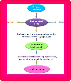
Fig. The engineering problem: solving process.)

where the dependent variable is a characteristic that usually reflects the behavior or state of the system; the independent variable are usually dimensions, such as time and space, along wich the system's behavior is being determined; the parameters are reflective of the system's properties or composition; and the forcing functions are external influences acting upon the system.

The actual mathematical expression of Eq. (1) can range from a simple algebraic relationship to large complicated sets of differential equations. For example, on the basis of his observations, Newton formulated his second law of motion, which states that the time rate of change of momentum of a body is equal to the resultant force acting on it. The mathematical expression, or model,

of the second law is the well-known equation

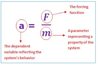
F = m.a (Eq (2))

where F = net force acting on the body, m = mass of the object, and a = its acceleration.

The second law can be recast in the format of Eq (1) by merely dividing both sides by m to give

Characteristics that are typical of mathematical models of the physical world:

1. It describes a natural process or system in mathematical terms.

2. It represents an idealization and simplification of reality. That is, the model ignores negligible details of the natural process and focuses on its essential manifestations. Thus, the second law does not include the effects of relativity that are minimal importance when applied to objects and forces that interact on or about the earth's surface at velocities and on scales visible to humans.

3. Finally, it yields reproducible results and, consequently, can be used for predictive purposes.

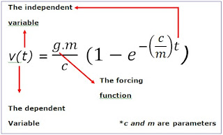
This equation, is called an analytical, or exact, solution because it exactly satisfies the original differential equation. Unfortunately, there are many mathematical models that cannot be solved exactly. In many of these cases, the only alternative is to develop a numerical solution that approximates the exact solution.

As conclution, numerical methods are those in wich the matematical problem is reformulated so it can be solved by arithmetic operations.


Source:
Numerical methods for Engineers
Fifth Edition
Steven C. Chapra
Raymond P. Canale
Mc Graw Hill

Model Types

Source: Métodos numéricos en ingeniería/
Capítulo I/Elkin Santafe/
Elementos básicos de modelamiento matemático

Welcome!! :)

Welcome to Numerical Methods Blog!
This is a space for you!On these days I will upload some contents about numerical methods. Wait for them! Ask what you want, I will try to answer to you.